Pre-Seismic Signature Detection using Diurnal GPS-TEC and Kriging Interpolation Maps (ASK-VTEC Technique):
11 May 2011, M9.0 Tohoku Earthquake Case Study

Thammaboribal P.,¹* Tripathi, N. K. ¹ and Lipiloet, S.²

¹Asian Institute of Technology, School of Engineering and Technology, P.O. Box 4, Klong Luang, Pathumthani 12120, Thailand

prapasgnss@gmail.com*

²Department of Civil Engineering, Faculty of Engineering, Rajamangala University of Technology Thanyaburi, Pathumthani 12120, Thailand

*Corresponding Author

Abstract

During earthquake preparation, a seismogenic electric field is generated on the Earth's surface, which then penetrates the atmosphere, reaching several hundred kilometers above the lithosphere and causing perturbations in the ionospheric electron density. These seismo-ionospheric anomalies are typically identified using statistical techniques, such as running averages or inter-quartile range (IQR), with the anomalous zones analyzed from Global Ionospheric Maps (GIMs). This study used ASK-VTEC technique for detecting pre-seismic signatures, based on the daily mean of vertical total electron content (AVTEC) and its standard deviation (SVTEC). The spatial distribution of vertical electron density (VTEC) is mapped using Ordinary Kriging (OrK) interpolation instead of GIMs. To validate and assess the performance of this approach, the M9.0 Tohoku earthquake, which occurred on March 11, 2011, was chosen as a case study. The results show that ionospheric anomalies were observed on May 8, 2011, three days before the earthquake. A significant anomalous zone was detected southwest of the epicenter between 06:00 and 10:00 UTC. These findings are consistent with previous studies, and further, the VTEC spatial distribution maps generated by the OrK interpolation technique outperformed GIMs on a local scale. Additionally, the analytical process is less complex compared to conventional methods. Therefore, the pre-seismic signature detection technique proposed in this study offers a viable alternative for investigating VTEC anomalies prior to earthquake events.

Keywords: ASK-VTEC, Earthquake Precursor, Ionospheric Disturbance, SVTEC, Tohoku Earthquake

1. Introduction

Seismo-ionospheric anomalies prior to earthquake occurrence were first detected in 1964 after the Mw 9.2 Alaska earthquake [1]. The study of ionospheric perturbations before earthquakes has been intensively conducted for many earthquake events. The results show that seismo-ionospheric anomalies typically emerge 0 to 10 days before an earthquake [2][3] and [4]. However, some scientists argue that there is no significant statistical relationship between the lithosphere, atmosphere, and ionosphere (LAI) during the earthquake preparation process [3]. As a result, the topic of ionospheric disturbances before earthquakes remains controversial and is still debated among seismologists. The physical mechanism of LAI coupling is not yet fully understood and continues to be discussed by many researchers. However, there are three hypotheses explaining this mechanism [4] and [5]. The first hypothesis is the chemical channel, based on the emanation of radon gas. The second hypothesis involves acoustic gravity waves (AGWs) generated during the earthquake preparation process, which may propagate upward to the ionosphere and cause irregularities in electron density [6]. The third hypothesis is the electro magnetic channel, which involves positive charge carriers [7]. The electrostatic electric field generated by positively charged ions at the Earth's surface penetrates through the atmosphere to the ionosphere, causing perturbations in electron density [8]. This theory is supported by a laboratory experiment that demonstrated that when rock samples are subjected to high stress, electrical charges are produced, flowing from the stressed part of the rock to the unstressed part. This process ionizes the air at the rock surface, resulting in changes in the conductivity of the air around the rock [9].

On a global scale, when rocks are stressed during the earthquake preparation process, positive charge carriers (holes) are released, traveling to the unstressed part of the rock and ionizing the near-ground atmosphere. This leads to changes in air conductivity due to the production of positive ions, which then penetrate through the atmosphere to the ionosphere, causing variations in electron density [10]. However, some laboratory experiments conducted by other researchers do not support the P-hole theory, as they argue that the Earth's crust is fluid-saturated, making it unlikely for electrical charge buildup to occur during the earthquake preparation process [11].

Seismo-ionospheric coupling is one of the candidates for investigating earthquake precursory signals. Increasingly, studies on this topic have been conducted using both ground-based stations and satellite data to confirm such mechanisms. The most widely used technique for detecting seismo-ionospheric anomalies prior to earthquakes is a statistical-based analytical technique, such as sliding median combined with interquartile range (IQR), which is used to construct upper and lower boundaries for detecting ionospheric anomalies [8][9][10][11][12] and [13]. Other techniques, such as artificial neural networks (ANN) [14][15] and [16], Particle Swarm Optimization (PSO) [17], radon anomalies [18], and very low frequency (VLF) radio waves [19], are also utilized. The most commonly used detection technique is the statistical-based method, where the threshold is set to median ± 2IQR. In cases where the observed VTEC lies very close to the threshold, it becomes questionable whether the value can be considered an anomaly.

The spatial distribution of total electron content (TEC) on a global scale is illustrated by Global Ionospheric Maps (GIMs), which are modeled using mathematical functions, such as spherical harmonic (SH) expansion. The spatial resolution of GIMs is 2.5° × 5° in latitude and longitude, respectively [12], and the temporal resolution is 2 hours. Since 1° at the equator corresponds to approximately 110 km and 95 km in latitude and longitude, respectively [13], the spatial resolution of GIMs at the equator is about 275 km in latitude and 475 km in longitude. For this reason, local ionospheric distribution cannot be accurately reproduced by GIMs [20], especially within the earthquake preparation zone. The distribution of vertical electron content (VTEC) can also be estimated from VTEC values at a set of reference GNSS stations using a "grid-based" technique, such as spatial interpolation. Many studies indicate that the VTEC instantaneous maps generated by the grid-based technique are roughly equivalent to, or even better than, the mathematical function-based technique [21] and [22], and they also show high accuracy when compared to the final product provided by the CODE analysis center [23].

Thus, in this study, the spatial distribution of VTEC maps was created by applying the "ordinary Kriging" interpolation technique to illustrate the variations in AVTEC and SVTEC values over the study area, instead of using GIMs. The performance of the interpolated maps was evaluated by collecting data from the Crustal Movement Observation Network of China (CMONOC) and the International GNSS Service (IGS) from DOY60 to DOY90 of 2015. Ordinary Kriging (OrK), Universal Kriging (UrK), inverse distance weighting (IDW) [24], and planar fit interpolation techniques were used to model regional VTEC maps in China. The results showed that the performance of UrK and OrK were similar, and both interpolation techniques produced better results than IGS GIMs when applied for ionospheric correction in GPS positioning. Moreover, OrK is particularly suitable for creating surface maps on a local scale [18].

To validate the performance of seismo-ionospheric anomaly detection using the ASK-VTEC technique [25] and ordinary Kriging interpolation maps, the M9.0 earthquake, known as the "Tohoku-Oki earthquake," was selected as a case study. This earthquake was chosen because studies on seismo-ionospheric anomaly detection related to this event have been widely reported. The submarine earthquake struck the east coast of Honshu, Japan, on March 11, 2011, at 05:46:23 UT. The epicenter was located at 38.927°N and 142.373°E in latitude and longitude, respectively. The focal depth of the earthquake was 29.0 km, which is considered a shallow earthquake. Previous studies show that anomalies related to this earthquake were observed as early as May 8, 2011, 0 to 4 days prior to the earthquake [26] and [27]. Therefore, the consistency of the anomalous days detected by the alternative techniques proposed in this study can be verified to determine whether the results correspond with those of previous studies.

2. Data and Methodology

The accuracy of GNSS measurements can be improved by eliminating or minimizing sources of error during the measurement process [28]v[29] and [30]. One of the largest sources of error is the electron density in the ionosphere, where the speed of the signals is delayed by particle charges. To minimize this error, it is necessary to measure the electron density in the ionosphere. A dual-frequency GNSS receiver receives L1 and L2 signals transmitted from navigation satellites in space.

The electron density in the ionosphere, known as the "total electron content" (TEC), along the signal path (STEC), is determined by the difference in the travel times of both signals from the satellite to the receiver, which is referred to as the "ionospheric time delay," as shown in Equation 1 [31].

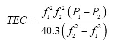
Equation 1

Where f₁ and f₂ are the frequencies of L₁ and L₂ signal which equal to 1575.42 MHz and 1227.60 MHz, respectively, P₁ and P₂ are the pseudo range measurements of L₁ and L₂ signal, respectively. TEC value derived from Equation (1) is the electron density along the ray path between the satellite and receiver so that it is called "slant TEC (STEC)". STEC can be converted to vertical total electron content (VTEC) at the pierce point of the ray path by Equation 2 [32]:

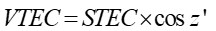
Equation 2

Where z' is zenith angle of satellite which is expressed in Equation 3:

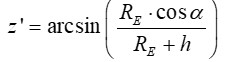
Equation 3

Where R_E is the radius of the earth which approximately equal to 6375 km; α is the GPS satellite elevation angle; and h is height of iono- spheric layer based on thin-shell theory, which is 350 km in this study. The unit of TEC is expressed as TECU (1 TECU = 10¹⁶ electrons/m²). The measured pseudo ranges contain bias values both in satellites and receiver so called "differential code bias (DCB)". The receiver contains larger DCB than that of the satellites, thus, the TEC estimation is affected by receiver DCB than satellite DCB [33]. The DCB values of reference stations can be obtained from ftp://ftp.aiub.unibe.ch/CODE, provided by the university of Bern, thus, equation 2 can be rewritten as in Equation 4 [34].

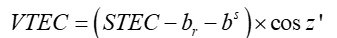
Equation 4

Where b_r and b^s are DCB values of receiver and satellite, respectively.

The earthquake preparation zone (EPZ) is determined as per Equation 5 [35] :

R = 10^0.43M

Equation 5

Where R is the radius of earthquake preparation area [km] and Mis the moment magnitude of earthquake.

2.1 Data Collection Data Processing and

Methodology

The moment magnitude of the earthquake is M9.0, according to Equation 5 the radius of EPZ is equivalent to 7,413 km. The boundary of EPZ was created by applying buffer operation as illustrates in Figure 1.

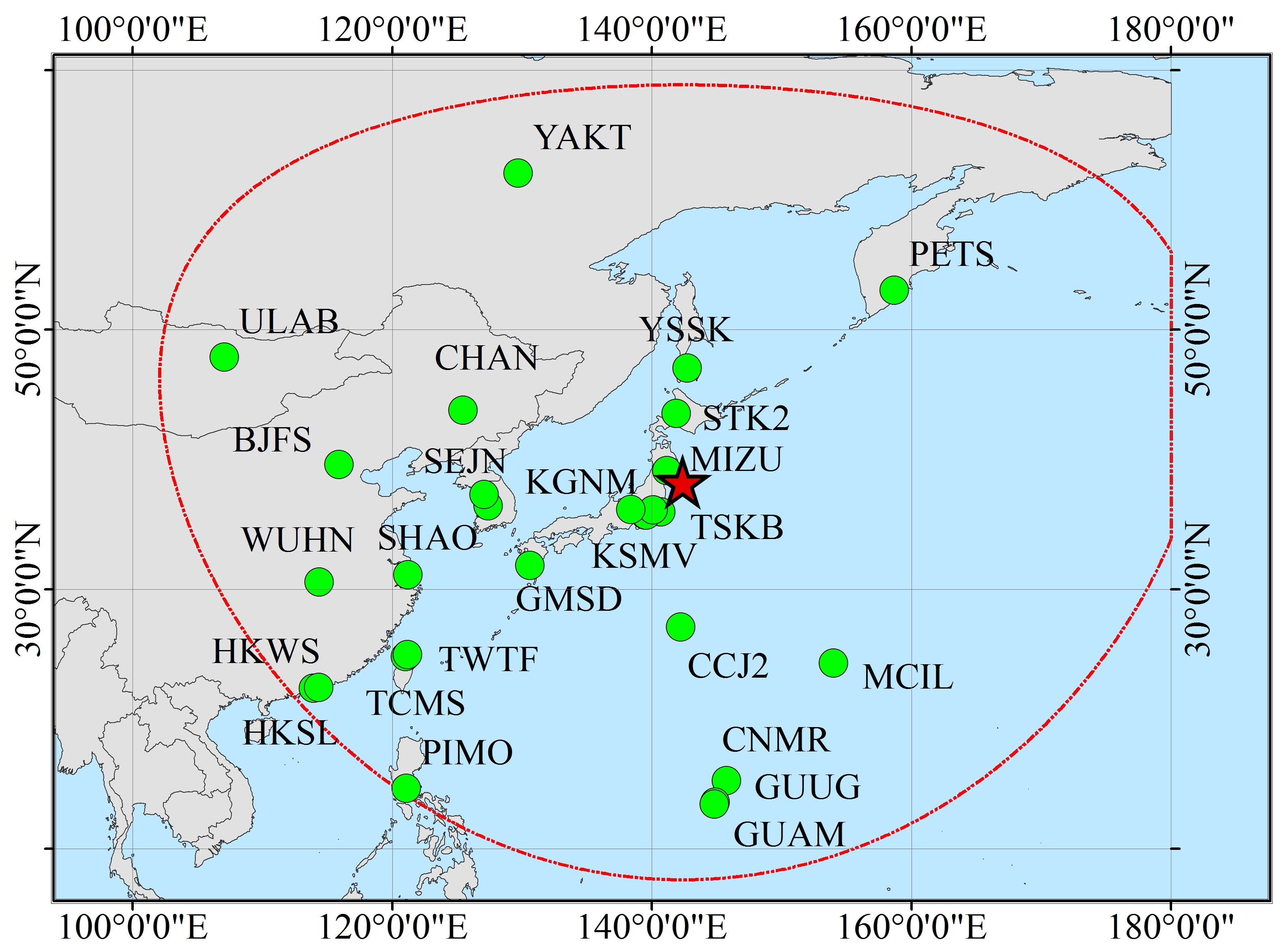
Figure 1 Earthquake preparation zone and selected IGS for data collection. Red solid star represents the earthquake epicenter, green solid circle represents IGS reference stations and red circle represents EPZ

Table 1: Selected IGS reference stations for data collection

The data were collected from the International GNSS service (IGS) reference stations that locate within the earthquake preparation zone as shown in Figure 1. In this study, the data from 29 IGS reference stations were collected, the list of the collected data illustrate in Table 1. The Receiver Independent Exchange Observation (RINEX.o) files for 10 days before and 5 days after the event were collected from the stations listed in Table 1. Previous studies have shown that anomalies were observed on March 8, 2011, which is 3 days prior to the earthquake event. Therefore, the performance of the ionospheric anomaly detection method proposed in this study can be validated. The data can be accessed at ftp://cddis.gsfc.nasa.gov/ gnss/data/daily. The daily data were recorded from 00:00:00 to 23:59:30 UTC with a sampling rate of 30 seconds. The data were processed using the open-source software "GPS-TEC," developed by Gopi Seemala, and only the GPS-TEC values were analyzed. The outputs from the software include both Slant Total Electron Content (STEC) and Vertical Total Electron Content (VTEC); however, only the VTEC values were analyzed. The daily mean of VTEC (AVTEC) and the standard deviation of VTEC (SVTEC) at each reference station were determined using the following equations:

The daily mean of VTEC (AVTEC) as well as standard deviation of VTEC (SVTEC) at each reference station were determined from Equations 6 and 7 [25].

Equation 6

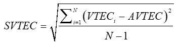
Equation 7

Where AVTEC is the average of VTEC on day-to-day basis, SVTEC is the standard deviation of AVTEC, N is the total number of measured VTEC from 00:00:00 to 23:59:30.

The ionospheric anomalies were detected from the variation plots of AVTEC and SVTEC. Both values were calculated on a day-to-day basis to ensure that they were not influenced by the TEC values of previous days. This anomaly detection technique is relatively straightforward and less complicated to implement compared to conventional techniques, such as the sliding median approach.

The ionospheric anomalies were further investigated by analyzing the spatial distribution of AVTEC and SVTEC, which were created using the ordinary Kriging interpolation technique. This technique is advantageous because, unlike deterministic interpolation methods that rely solely on values within the search radius, it also accounts for statistical relationships, such as spatial autocorrelation, in surface generation. In this study, the variation of VTEC over the study area, typically presented by GIMs, was replaced by AVTEC and SVTEC maps. To investigate the day-to-day variations in VTEC prior to the Tohoku earthquake, interpolated maps were created for the 10 days and 5 days before and after the event. Although a running window of 27 days is typically required to account for periodic changes due to the short-period oscillation of the ionosphere, previous studies on this earthquake case showed that anomalies were observed 0-4 days prior to the event. Since the main objective of this study is to propose an alternative VTEC anomaly detection approach based on diurnal VTEC, the 10-day and 5-day periods before and after the event were sufficient to validate whether the results are consistent with previous studies that used conventional detection techniques.

Although the temporal resolution of GIMs is 2 hours [26], the temporal resolution of AVTEC and SVTEC maps was set to 1 day as a rough anomaly scanner. This is because anomalous days can be detected by significantly high variations in AVTEC/SVTEC compared to previous days. With this assumption, the variation of VTEC is not influenced or disturbed by VTEC variations from prior days. The duration of TEC anomalies during the earthquake preparation period is typically 4-6 hours on anomalous days [26] and [36].

Table 2: Sources of solar activity index and geomagnetic storm indices

Based on statistical theory, the distribution characteristics of VTEC values on anomalous days would change due to disturbances in the dataset caused by the seismo-ionospheric mechanism. Therefore, the diurnal VTEC (AVTEC) and its standard deviation (SVTEC) on anomalous days are significantly different from those on other days. According to this statistical assumption, it is possible to investigate VTEC anomalies using AVTEC and SVTEC. Finally, the AVTEC/SVTEC variation maps, with a temporal resolution of 2 hours (similar to GIMs), were analyzed on anomalous days to investigate whether an anomalous zone appears within the EPZ.

2.2 Influence of Geomagnetic Storms and Solar Activity to Ionospheric Perturbation

Ionospheric TEC disturbance is mostly associated with space weathers, so the influence of the space weather on detected anomalous day must be investigated in order to determine whether the detected anomaly is attributed to space weathers or earthquake preparation process. The magnitude of geomagnetic activity is measured by two indicators as disturbance storm time index (Dst) and geomagnetic index (Kp). Solar activity magnitude is presented by solar radio flux at 10.7 cm index (F10.7). These three indices can be achieved from the links given in Table 2. It is difficult to determine whether the anomaly is induced by the influence of an earthquake or space weather [37] and [38]. The three indices listed in Table 2 were used to distinguish whether the anomaly was caused by a seismo-ionospheric event, space activities, or a geomagnetic storm. If the solar-geomagnetic index exceeds the following limits: |Dst| index < 30 nT, Kp index > 3, and F10.7 > 150.

2.3 Ordinary Kriging Interpolation (ORK)

The variation of VTEC was illustrates by AVTEC and SVTEC maps, the maps were created by applying geostatistical interpolation technique so called "Ordinary Kriging (OrK)", this technique is successfully applied to obtain ionospheric information in SBAS, WAAS or GAGAN [39]. The assigned weights in this interpolation technique are not only relied on the distances between unknown points and measured points but spatial autocorrelation is also taken account in the weight determination, so that it gives the best linear unbiased prediction values [40][41] and [42]. The prediction values Z(x₀) at any locations within the study were determined from the known values Z(x_i) , and the weights that derived from variogram as summarized by Equation 8:

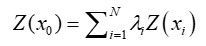
Equation 8

Where Z(x₀) is the prediction value at x₀location, Z(x_i) is the known values that obtained at x_ilocation which is AVTEC and SVTEC at x _i location in this study, and is the weight function that depends on the semivariogram, the distance between prediction and known point, and the spatial relationship among the known values around the prediction point. The determination of the weights is based on minimizing the variance of the variable as per Equation 9.

Var(Z(x + h) – z(x)) = 2γ(|h|)

Equation 9

Where var is the variance function, x and x+h are two adjacent locations and γ represents the variogram. The expectation of Z(x+h) and Z(x) is defined in Equation 10.

E(Z(x + h) – z(x)) = 0

Equation 10

Where E is the expectation operator.

In order to satisfy the unbiasness in the prediction, the difference between the predictions and true values should be zero. To ensure that the predictors are unbias for unknown measurement, the sum of the weight equal to 1 is imposed as Equation 11.

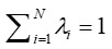
Equation 11

The solution to the minimization, constrained by unbiasness is done by applying Lagrange method, and the kriging equation is expressed as a matrix in Equations 12 and 13.

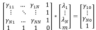
Equation 12

Equation 13

3. Results

The outputs derived from data processing using GPS-TEC software contain slant TEC (STEC) as well as VTEC values. In this study, only VTEC is analyzed and discussed. The AVTEC and SVTEC at each reference station on daily basis were determined.

3.1 Average Diurnal Vertical Total Electron Content (AVTEC)

AVTEC of 10 days before and 5 days after the earthquake events were plotted for investigating the variation of diurnal VTEC. The variation of AVTEC of 29 IGS stations illustrates in Figure 2. The figure shows the variation of AVTEC at each IGS reference station from DOY060 to DOY075. It can be seen that high variations of AVTEC were observed on DOY062, DOY064, and DOY067, which are 8 days, 6 days, and 3 days prior to the earthquake occurrence, respectively. Periodic oscillations were observed at the TCMS and TWTF stations, both located southwest of the epicenter. Although the expected normal level of AVTEC at each station is not known, and it is difficult to define what can be considered an anomaly, Figure 2 displays that anomalous AVTEC values were observed at both stations. After DOY067, it is clearly seen that the AVTEC at both stations decreased, and high variations were no longer observed. The average AVTEC from DOY060 to DOY066 at TCMS and TWTF were 18.98 TECU and 18.63 TECU, respectively, while the maximum AVTEC values observed on DOY067 were 31.36 TECU and 31.38 TECU, respectively. The peak of AVTEC at some stations within the EPZ was also observed on DOY062, DOY064, and DOY067, but the latter day showed a significant high variation of AVTEC. The AVTEC variations in the northern part of the study area showed a flat behavior, and the AVTEC values were relatively low compared to the southern part.

The AVTEC at PIMO also showed a high value compared to the other stations. The AVTEC at PIMO gradually increased from 20.48 TECU on DOY060 and reached its peak of 33.02 TECU on DOY071. The variation of AVTEC at GUUG, GUAM, and CNMR, which are located at the same latitude as PIMO, exhibited the same behavior as at PIMO. However, periodic oscillations were not observed as they were at TCMS and TWTF. To investigate the spatial distribution of AVTEC over the study area, time series AVTEC maps from DOY060 to DOY075 (1–16 May 2011) were created using the ordinary Kriging interpolation technique. The time series map of AVTEC is illustrated in Figure 3. The spatial distribution of AVTEC over the study area, illustrated in Figure 3, clearly shows that the AVTEC at lower latitudes contains higher AVTEC values than those at higher latitudes. This is because the electron density along these latitudes is influenced by the northern crest of the equatorial fountain, which occurs only during the daytime. AVTEC anomalies were significantly observed on DOY064 and DOY067 in the southwest of the epicenter.

Figure 2: TEC anomaly detection from diurnal AVTEC.
Red star represents the day of earthquake event

Figure 3: Time-series map of AVTEC from May 1, 2011 to May 16, 2011 (DOY060 to DOY075).
Red solid star represents the earthquake epicenter

However, it is difficult to determine whether the AVTEC anomalies on these days could be considered pre-seismic signatures of the Tohoku earthquake, as the anomalous zone remained in the southwest of the epicenter even after the earthquake occurred. The interpolated maps reveal that the distribution of AVTEC in the study area was mainly influenced by the AVTEC values at the IGS stations located at lower latitudes.

3.2 Standard Deviation of Diurnal Vertical Total Electron Content (SVTEC)

According to the previous studies, on the anomalous day, the VTEC anomalies occurred between 12:00LT and 18:00LT with the duration of about 2 hours, so that the electron content was likely to be disturbed by the exceeding particle charges generated by earthquake preparation process and caused the variation in data distribution. The assumption of the VTEC anomaly detection derives from the daily standard deviation of VTEC (SVTEC) is that an abnormal peak of SVTEC will be observed on the anomalous day because the standard deviation of VTEC on anomalous day should be higher than the ordinary days. The time series distribution plot of SVTEC 10 days before and 5 days after the earthquake illustrates in Figure 4.

Figure 4 illustrates that the characteristics of SVTEC oscillation are similar to those of AVTEC, with abnormal peaks observed on DOY062, DOY064, and DOY067, which were 8 days, 6 days, and 3 days prior to the earthquake occurrence, respectively. The maximum SVTEC values appeared at TCMS and TWTF on DOY067. Since the distance between these two IGS reference stations is approximately 24.76 km, the difference in SVTEC values between the stations was a maximum of 0.57 TECU. The SVTEC at HKWS and HKSL was also higher compared to the other stations on DOY067, but no significant variation in SVTEC at these stations was observed. The average SVTEC from DOY060 to DOY066 at TCMS and TWTF was 15.17 TECU and 14.98 TECU, respectively, while the maximum SVTEC values observed on DOY067 were 24.31 TECU and 24.15 TECU, respectively.

Figure 4: TEC anomaly detection from diurnal SVTEC.
Red star represents the day of earthquake event

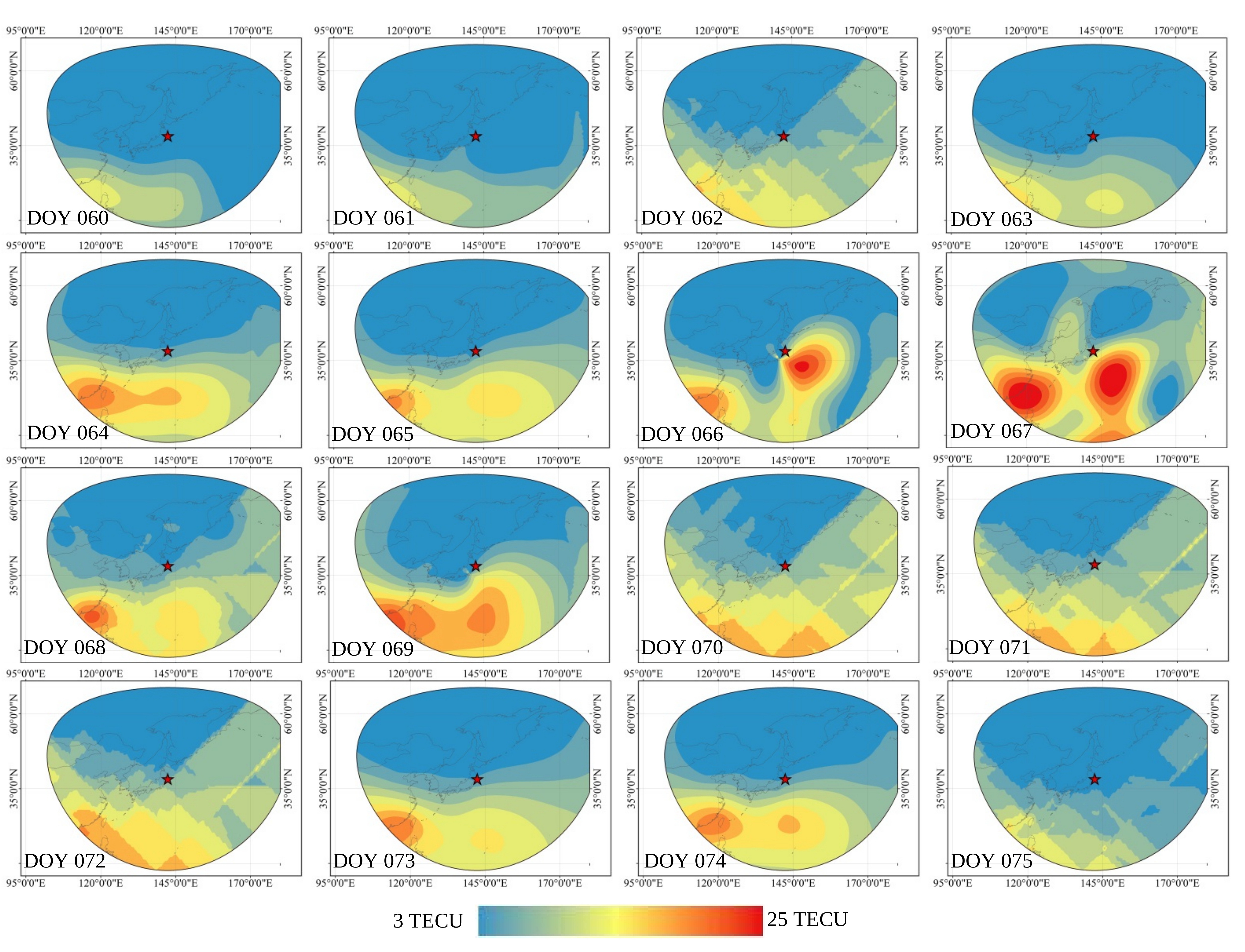
Figure 5: Time-series map of SVTEC from May 1, 2011 to May 16, 2011 (DOY060 to DOY075)
Red solid star represents the earthquake epicenter

Thus, the high variations in SVTEC on DOY067 are likely to be considered as SVTEC anomalies prior to the Tohoku earthquake. To investigate the spatial variations of SVTEC over the study area, a statistical interpolation technique called "Ordinary Kriging" was used to generate SVTEC distribution maps. The maps were generated on a day-to-day basis to identify the anomalous days. The time series of SVTEC spatial distribution from DOY060 to DOY075 (May 1, 2011, to May 16, 2011) is illustrated in Figure 5. The spatial distribution of SVTEC in Figure 5 shows that the characteristics of SVTEC variation were similar to those of AVTEC, with SVTEC concentration inversely proportional to latitude.

Figure 6: Spatial distribution of regional VTEC from 02:00UT to 24:00 UT on March 8, 2008
Red solid star represents the earthquake epicenter

However, the abnormal SVTEC zone was more significant than the AVTEC zone. According to Figure 5, the SVTEC anomalous zone was first observed on DOY064 in the southwest of the epicenter, the same region as the AVTEC anomaly. The anomalous zone then clearly reappeared in the southeast direction of the epicenter on DOY066 and reached its peak value on DOY067. Thus, it is suspected that the SVTEC anomalies on DOY066 and DOY067 were most likely associated with the Tohoku earthquake, as the anomalous zone was located very close to the earthquake epicenter.

To assess the performance of the AVTEC and SVTEC distribution maps modeled by the Ordinary Kriging Interpolation (OrK) technique, the VTEC on DOY067 (the anomalous day) was created with a temporal resolution of two hours, as GIMs. This allows the consistency of the results between the interpolated maps and GIMs to be evaluated. The output maps are illustrated in Figure 6. Basically, the distribution of VTEC is presented by global ionospheric maps (GIMs) generated from IGS-GPS data with spherical harmonic expansion and is utilized for identifying VTEC anomalous zones. However, in this study, GIMs were replaced by OrK-interpolated maps with the same temporal resolution of two hours as the GIMs. Figure 6 shows the variation of VTEC on the anomalous day (May 8, 2011) from 02:00 UT to 24:00 UT. It is clearly seen that VTEC started increasing from 06:00 UT, reached its maximum level from 08:00 UT to 10:00 UT, and gradually decreased afterward. The anomalous zone was located in the southwest of the epicenter, in the same region as the AVTEC and SVTEC anomalous zones on DOY067. In terms of time and space, the results are consistent with previous studies [27] and [43]. Thus, it is reasonable to infer that the VTEC distribution can be represented by OrK-interpolated maps because they provide equivalent or even better output maps compared to GIMs.

3.3 Influence of Solar Activity and Geomagnetic Storm

The electron density in the ionosphere is normally affected by solar activities and geomagnetic storms. Therefore, the levels of both phenomena on the anomalous days were monitored to investigate whether the VTEC anomaly is attributed to such phenomena or to the earthquake preparation process. The magnitude of geomagnetic activity is indicated by two indices: the disturbance storm time index (Dst) and the geomagnetic index (Kp). When the ionosphere is disturbed by a geomagnetic storm, the values of |Dst| < 30 nT and Kp > 3 are observed. The magnitude of solar activity is indicated by the solar radio flux at the 10.7 cm index (F10.7). If the index is greater than 150 SFU, it indicates that the ionosphere is disturbed by solar activities.

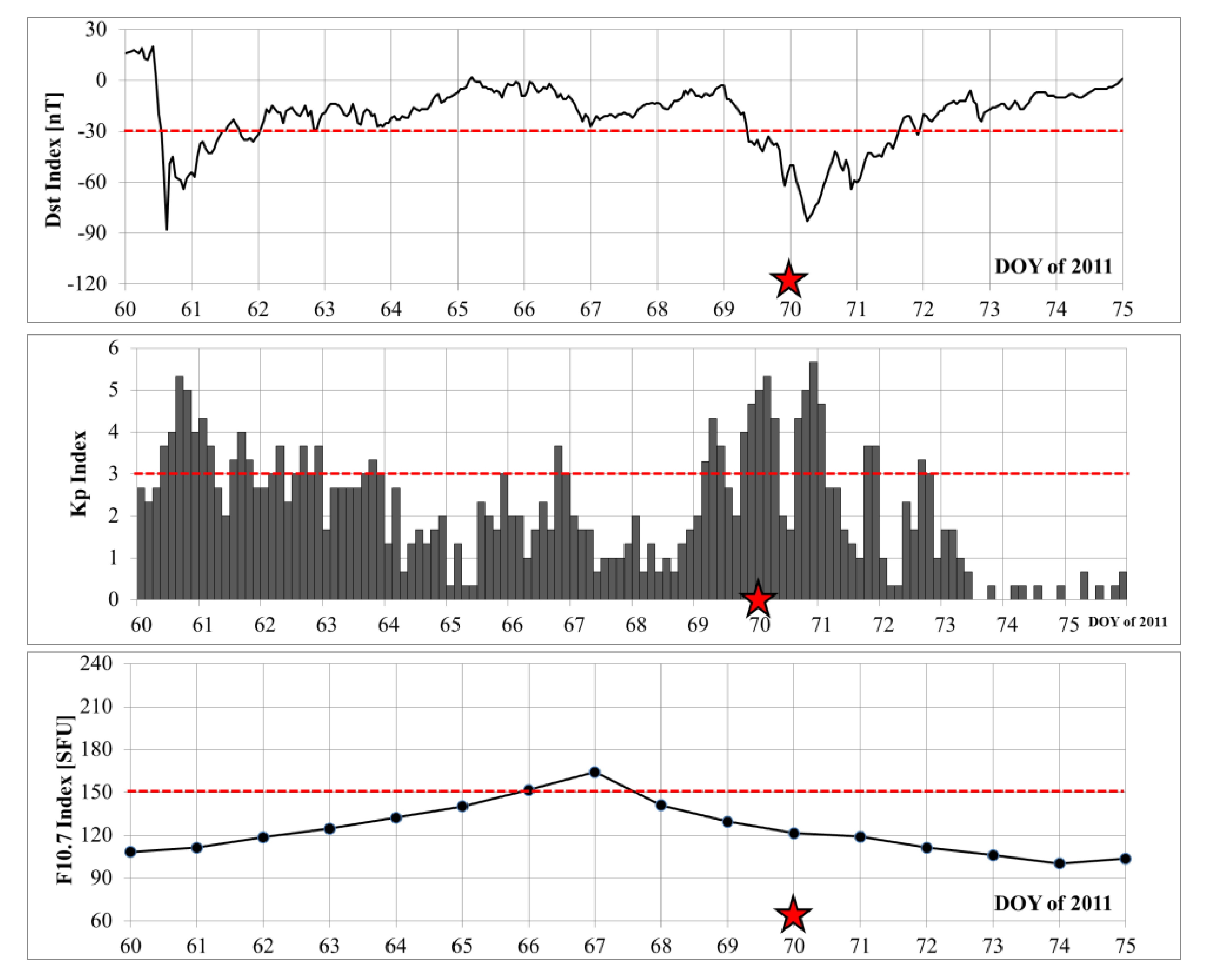
Figure 7: Variations of geomagnetic storm indices ( Dst and Kp) and solar activity index (F10.7) from DOY060 to DOY 075 (May 1, 2011 to May 16, 2011)
red sold star represents Tohoku earthquake event day,
and red dashed line represents geomagnetic storm and solar activity thresholds

References

[1] Davies, K. and Baker, D. M., (1965). Ionospheric Effects Observed
Around the Time of the Alaskan Earthquake of March 28, 1964.
Journal of Geophysical Research
, Vol. 70(1965), 2251–2253.
https://doi.org/10.1029/JZ070i009p02251.
[2] Tojiev, S. R., Ahmedov, B. J., Tillayev, Y. A. and Eshkuvatov, H.
E., (2013). Ionospheric Anomalies of Local Earthquakes Detected by GPS TEC
Measurements Using Data from Tashkent and Kitab Stations.
Advances in Space Research
, Vol. 52(6), 1146–1154.
https://doi.org/10.1016/j.asr.2013.06.011.
[3] Dautermann, T., Calais, J., E. and Haase, J., (2007). Garrison,
Investigation of Ionospheric Electron Content Variations Before Earthquakes
in Southern California, 2003-2004,
Journal of Geophysical Research: Solid Earth
, Vol. 112(B2), 2003–2004.
https://doi.org/10.1029/2006JB004447.
[4] Hayakawa, M., (2016). Earthquake Prediction with Electromagnetic
Phenomena. AIP Conference Proceedings, Vol. 1709(1).
https://doi.org/10.1063/1.4941201.
[5] Li, M., Kong, W., Yue, C., Song, S., Yu, C., Xie, T. and Lu, X.,
(2018). An Estimation of "Energy" Magnitude Associated with a Possible
Lithosphere-Atmosphere-Ionosphere Electro-magnetic Coupling Before the
Wenchuan MS8.0 Earthquake.
Earthquakes - Forecast, Prognosis and Earthquake Resistant Construction
.
https://doi.org/10.5772/intechopen.75880.
[6] Piersanti, M., Materassi, M., Battiston, R., Carbone, V., Cicone,
A., D'Angelo, G., Diego, P. and Ubertini, P., (2020).
Magnetospheric–Ionospheric–Lithospheric Coupling Model. 1: Observations
During the 5 August 2018 Bayan Earthquake. Remote Sensing, Vol.
12, 1–25.
https://doi.org/10.3390/rs12203299.
[7] Freund, F., (2013). Earthquake Forewarning - A Multidisciplinary
Challenge from the Ground up to Space. Acta Geophysica, Vol. 61(4).
https://doi.org/10.2478/s11600-0130130-4.
[8] Yan, X., Yu, T., Shan, X. and Xia, C., (2017). Ionospheric TEC
Disturbance Study Over Seismically Region in China.
, Vol. 60(12), 2822–2835.
https://doi.org/10.1016/j.asr.2016.12.004.
[9] Freund, F., T., Kulahci, I., G., Cyr, G., Ling, J., Winnick, M.,
Tregloan-Reed, J. and Freund, M. M., (2009). Air Ionization at Rock Surfaces
and Pre-Earthquake Signals.
Journal of Atmospheric and Solar-Terrestrial Physics
, Vol. 71(17), 1824–1834.
https://doi.org/10.1016/j.jastp.2009.07.013.
[10] Sharma, G., Champati Ray, P., K., Mohanty, S. and Kannaujiya, S.,
(2017). Ionospheric TEC Modelling for Earthquakes Precursors from GNSS Data.
Quaternary International, Vol. 462, 65–74.
https://doi.org/10.1016/j.quaint.2017.05.007.
[11] Dahlgren, R. P., Johnston, M. J. S., Vanderbilt, V. C. and Nakaba, R.
N., (2014). Comparison of the Stress-Stimulated Current of Dry and
Fluid-Saturated Gabbro Samples.
Bulletin of the Seismological Society of America
, Vol. 104(6), 2662–2672.
https://doi.org/10.1785/0120140144.
[12] Devi̇Ren, M. N. and Arikan, F., (2018). IONOLAB-MAP: An Automatic
Spatial Interpolation Algorithm for Total Electron Content.
Turkish Journal of Electrical Engineering and Computer Sciences
, Vol. 26(4), 1933–1945.
https://doi.org/10.3906/elk1611-231.
[13] Liu, J. Y., Chen, Y. I., Chen, C. H., Liu, C. Y., Chen, C. Y.,
Nishihashi, M., Li, J. Z., Xia, Y. Q., Oyama, K. I., Hattori, K. and Lin, C.
H., (2009). Seismoionospheric GPS Total Electron Content Anomalies Observed
before the 12 May 2008 Mw7.9 Wenchuan Earthquake.
Journal of Geophysical Research: Space Physics
, Vol. 114(A04320), 1–10.
https://doi.org/10.1029/2008JA013698
[14] Thammaboribal, P. and Tripathi, N. K., (2024). Predicting Land Use
and Land Cover Changes in Pathumthani, Thailand: A Comprehensive Analysis
from 2013 to 2023 Using Landsat Satellite Imagery and CA-ANN Algorithm,
with Projections for 2028 and 2038.
International Journal of Geoinformatics
, Vol. 20(5), 13–27.
https://doi.org/10.52939/ijg.v20i5.3225.
[15] Paluang, P., Thavorntam, W. and Phairuang, W., (2024). Application of
Multilayer Perceptron Artificial Neural Network (MLP-ANN) Algorithm for
PM2.5 Mass Concentration Estimation during Open Biomass Burning Episodes in
Thailand. International Journal of Geoinformatics, Vol. 20(7),
28–42.
https://doi.org/10.52939/ijg.v20i7.3401.
[16] Benchelha, N., Bezza, M., Belbounaguia, N., Benchelha, S. and
Benchelha, M., (2022). Modeling Dynamic Urban Growth Using Cellular Automata
and Geospatial Technique: Case of Casablanca in Morocco.
, Vol. 18(5), 27–40.
https://doi.org/10.52939/ijg.v18i5.2369.
[17] Akhoondzadeh, M., (2014). Thermal and TEC Anomalies Detection Using
an Intelligent Hybrid System Around the Time of the Saravan, Iran, (M W =
7.7) Earthquake of 16 April 2013. Advances in Space Research, Vol.
53(4), 647–655.
https://doi.org/10.1016/j.asr.2013.12.017.
[18] Alam, A., Wang, N., Zhao, G. and Barkat, A., (2020). Implication of
Radon Monitoring for Earthquake Surveillance Using Statistical Techniques: A
Case Study of Wenchuan Earthquake. Geofluids, Vol. 2020.
https://doi.org/10.1155/2020/2429165.
[19] Pandey, U., Singh, A. K., Kumar, S. and Singh, A. K., (2018).
Seismogenic Ionospheric Anomalies Associated with the Strong Indonesian
Earthquake Occurred on 11 April 2012 (M = 8.5).
, Vol. 61(5), 1244–1253.
https://doi.org/10.1016/j.asr.2017.12.022.
[20] Wielgosz, P., Grejner-Brzezinska, D. and Kashani, I., (2003).
Regional Ionosphere Mapping with Kriging and Multiquadric Methods.
The Journal of Global Positioning Systems
, Vol. 2(1), 48–55.
https://doi.org/10.5081/jgps.2.1.48.
[21] Li, M., Yuan, Y., Wang, N., Li, Z., Liu, X. and Zhang, X., (2018).
Statistical Comparison of Various Interpolation Algorithms for
Reconstructing Regional Grid Ionospheric Maps Over China.
, Vol. 172, 129–137.
https://doi.org/10.1016/j.jastp.2018.03.017.
[22] Gao, Y. and Liu, Z. Z., (2002). Precise Ionosphere Modeling Using
Regional GPS Network Data.
, Vol. 1(1), 18–24.
https://doi.org/10.5081/jgps.1.1.18.
[23] Zhang, Q. and Wang, J., (2019). VTEC Reconstruction of the
Ionospheric Grid with Kriging Interpolation.
IOP Conference Series: Earth and Environmental Science
, Vol. 237(6).
https://doi.org/10.1088/1755-1315/237/6/062001.
[24] Ihsan, H., Astari, A., Bratanegara, A., Aliyan, S. and Wulandari, E.,
(2021). The Comparison of Spatial Models in Peak Ground Acceleration (PGA)
Study. International Journal of Geoinformatics, Vol. 17(6), 27–33.
https://doi.org/10.52939/ijg.v17i6.2061.
[25] Thammaboribal, P., Tripathi, N. K., Ninsawat, S. and Pal, I., (2022).
Earthquake Precursory Detection Using Diurnal GPS-TEC and Kriging
Interpolation Maps: 12 May 2008, Mw7.9 Wenchuan Case Study.
MethodsX
, Vol. 9.
https://doi.org/10.1016/j.mex.2022.101617.
[26] Fuying, Z. and Yun, W., (2011). Anomalous Variations in Ionospheric
TEC Prior to the 2011 Japan Ms9.0 Earthquake.
Geodesy and Geodynamics
, Vol. 2(3), 8–11.
https://doi.org/10.3724/sp.j.1246.2011.00008.
[27] Le, H., Liu, L., Liu, J., Y., Zhao, B., Chen, Y. and Wan, W., (2013).
The Ionospheric Anomalies Prior to the M9.0 Tohoku-Oki Earthquake.
Journal of Asian Earth Sciences
, Vol. 62, 476–484.
https://doi.org/10.1016/j.jseaes.2012.10.034.
[28] Fazilova, D., Makhmudov, M. and Magdiev, K., (2023). Analysis of
Crustal Movements in the Angren-Almalyk Mining Industrial Area Using GNSS
Data. International Journal of Geoinformatics, Vol. 19(11), 12–19.
https://doi.org/10.52939/ijg.v19i11.2915.
[29] Mustafin, M., Nasrullah, M. and Abboud, M., (2024). A Comparative
Analysis of GNSS Processing Services for Static Measurements: Evaluating
Accuracy and Stability at Different Observation Periods.
, Vol. 20(9), 112–121.
https://doi.org/10.52939/ijg.v20i9.3553.
[30] Kandil, I., Awad, A. and El-Mewafi, M., (2023). Role of
Multi-Constellation GNSS in the Mitigation of the Observation Errors and the
Enhancement of the Positioning Accuracy.
, Vol. 19(4), 25–35.
https://doi.org/10.52939/ijg.v19i4.2631.
[31] Blewitt, G., (1990). An Automatic Editing Algorithm for GPS Data.
Geophysical Research Letters, Vol. 17(3), 199–202.
https://doi.org/10.1029/GL017i003p00199.
[32] Ma, G. and Maruyama, T., (2003). Derivation of TEC and Estimation of
Instrumental Biases from GEONET in Japan. Annals of Geophysics,
Vol. 21(10), 2083–2093.
https://doi.org/10.5194/angeo-21-2083-2003.
[33] Choi, B. K., Lee, W. K., Cho, S. K., Park, J. U. and Park, P. H.,
(2010). Global GPS Ionospheric Modelling Using Spherical Harmonic: Expansion
Approach. Journal of Astronomy and Space Sciences, Vol. 27(4),
359–366.
https://doi.org/10.5140/JASS.2010.27.4.359.
[34] Schaer, S., (1999).
Mapping and Predicting the Earth's Ionosphere Using the Global
Positioning System, Institut für Geodäsie und Photogrammetrie
, Eidg. Technische Hochschule Zürich. [Online]. Available;
https://books.google.co.th/books?id=zinKAAAACAAJ"
[Accessed: Sep. 19, 2024].
[35] Dobrovolsky, I. P., Zubkov, S. I. and Miachkin, V. I., (1979).
Estimation of the Size of Earthquake Preparation Zones.
Pure and Applied Geophysics
, Vol. 117, 1025–1044.
https://doi.org/10.1007/BF00876083.
[36] Wang, L., Jinyun, G., Xuemin, Y. and Honguan, Y., (2014). Analysis of
Ionospheric Anomaly Preceding the Mw7. 3 Yutian Earthquake.
, Vol. 5(2), 54–60.
https://doi.org/10.3724/sp.j.1246.2014.02054.
[37] Zhu, F., Lin, J., Su, F. and Zhou, Y., (2016). A Spatial Analysis of
the Ionospheric TEC Anomalies Prior to M7.0+ Earthquakes during 2003–2014.
Advances in Space Research, Vol. 58(9), 1732–1738.
https://doi.org/10.1016/j.asr.2016.06.040"
[38] Jiang, W., Ma, Y., Zhou, X., Li, Z., An, X. and Wang, K., (2017).
Analysis of Ionospheric Vertical Total Electron Content before the 1 April
2014 Mw 8.2 Chile Earthquake. Journal of Seismology, Vol. 21,
1599–1612.
https://doi.org/10.1007/s10950-017-9684-y.
[39] Rodríguez-Bouza, M., Paparini, C., Otero, X., Herraiz, M., Radicella,
S. M., Abe, O. E. and Rodríguez-Caderot, G., (2017). Southern European
Ionospheric TEC Maps Based on Kriging Technique to Monitor Ionosphere
Behavior. Advances in Space Research, Vol. 60(8), 1606–1616.
https://doi.org/10.1016/j.asr.2017.05.008.
[40] Pantolla, H., Malay, C., Leonisa, M., Reyes Jr., R. and Legaspi, M.,
(2024). Geostatistical Exploration of Some Water Quality Clusters in Laguna
Lake, Philippines. International Journal of Geoinformatics, Vol.
20(4), 1–18.
https://doi.org/10.52939/ijg.v20i4.3143.
[41] Noinak, M., Charoenphon, C., Weerawong, K. and Satirapod, C., (2022).
Testing Horizontal Coordinate Correction Model Used for Transformation from
PPP GNSS Technique to Thai GNSS CORS Network Based on ITRF2014.
, Vol. 18(3), 55–64.
https://journals.sfu.ca/ijg/index.php/journal/article/view/2203.
[42] Charoenkalunyuta, T., Satirapod, C., Charoenyot, R. and Thongtan, T.,
(2023). Geometric and Statistical Assessments on Horizontal Positioning
Accuracy in Relation with GNSS CORS Triangulations of NRTK Positioning
Services in Thailand. International Journal of Geoinformatics,
Vol. 19(2), 1–9.
https://doi.org/10.52939/ijg.v19i2.2559.
[43] Jian, Y., Yiyan, Z. and Fanfan, S., (2012). Ionospheric Anomaly
before the 2011 Tohoku Mw 9.0 Earthquake. Geodesy and Geodynamics,
Vol. 3(3), 17–22.
https://doi.org/10.3724/sp.j.1246.2012.00017.
[44] Zhu, F., Zhou, Y. and Wu, Y., (2013). Anomalous Variation in GPS TEC
Prior to the 11 April 2012 Sumatra Earthquake.
Astrophysics and Space Science
, Vol. 345, 231–237.
https://doi.org/10.1007/s10509-0131389-2.