Multiscale Space-Time Analysis of Environmental Changes in the Oil Sands Area (Alberta, Canada)

Couloigner, I.,¹* Fallah, B., ¹ Hanes, A., ¹ Mirzaei, M., ² Dempsey, D. ¹ and Bertazzon, S.¹

¹Department of Geography, University of Calgary, Alberta, Canada

²EarthDaily Analytics, BC, Canada,

*Corresponding Author

Abstract

Our study encompasses the Oil Sands Area (OSA) within northern Alberta, Canada, which has experienced substantial environmental changes over the last decades, in association with natural and anthropogenic disturbances. Using composites of Landsat imagery for 5-year intervals between 2000 and 2020, we performed two parallel geospatial analyses to assess environmental changes, examining landscape metrics and spectral indices. Landscape metrics were calculated from land use/land cover maps derived from a Random Forest supervised classification. Spectral indices included Normalized Difference Vegetation Index (NDVI) and Normalised Difference Built-up Index (NDBI), among others. Both hierarchical zonal analysis of spectral indices and zonal landscape metrics were calculated based upon two different aggregations of nested drainage basin features from hydrologic unit code (HUC - Watersheds of Alberta). Spatial contiguity of changes was evaluated by hotspot analysis. HUCs determined to experience significant changes at coarse aggregation level were examined at finer level. The combination of landscape metrics and zonal analysis provided evidence of substantial, yet localized, areas of changing trends. Mixed forest experienced the most significant changes; urban/barren areas initially increased and later decreased, indicating change both in agricultural and human-made areas.

Keywords: Oil Sands Area, Environmental Changes, Hotspot Analysis, Landscape Metrics, LULC, Spectral Indices

1. Introduction

Environmental changes, sudden or gradual, can be complex. This complexity, compounded with the diversity of a region and the interconnections of its environmental drivers, may make it hard to clearly detect changes over a given area and time frame. Observed changes can be associated with physical and anthropogenic processes, interacting with the environment and with each other at varying spatial and temporal scales. The range of such dynamic processes includes both physical (i.e., climate change, forest fires, and floods), and anthropogenic ones (i.e., population and urban dynamics, or agricultural, industrial, and extraction activities), among others. At the ecosystem level, environmental changes can constitute disturbances; therefore, it is important not only to detect them, but also to quantify them, particularly in their spatial and temporal dimensions. Their detection and quantification form the basis for an improved understanding, monitoring, and managing of the ecosystem [1]. Our study area encompasses the Oil Sands Area (OSA) within northern Alberta. Sponsored by the Oil Sands Monitoring Program (Government of Alberta (GoA)), our project was designed to provide spatial and spatiotemporal information to support the monitoring and management of the area. The spatial extent of the OSA is just over 140,000 km², and it is subdivided into a series of drainage basins, used for management purposes, and further subdivided into hydrologic units from Hydrologic Unit Codes (HUCs) at several hierarchical levels [2].

The literature on environmental change detection covers a range of methods and approaches, which vary, in part, as a function of the size of the study area, the analytical scale, and the temporal scale, and are often subject to constraints, such as data availability or specific management needs [3][4][5][6][7][8][9][10] and [11].

Frequently, analyses are conducted within environmental indicator systems, such as the DPSIR (Driver-Pressure-State-Impact-Response)framework [12], which encompasses information about diverse, interconnected environmental drivers [13][14] and [15]. The choice of (any) analytical scale is also prone to the modifiable areal unit problem (MAUP), whereby analytical results vary depending on the scale and aggregation of spatial units [16] and [17]. Hence, while the MAUP cannot be solved or avoided, analytical results obtained for a given scale or aggregation should not be extrapolated to different ones.

The goal of this study was to analyze spatial and temporal environmental changes that can be associated with anthropogenic and natural disturbances in the OSA as a whole and throughout its HUCs. To this end, and cognisant of the MAUP, we developed an articulated geospatial and temporal analysis, which encompasses varying spatial scales and considers different dimensions of change. The spatiotemporal investigation was conducted through two, independent and complementary, analyses: (1) Temporal comparison of landscape and class metrics and (2) Hierarchical zonal analysis of spectral indices and zonal metrics. In the spatiotemporal analysis, these sequences of changes yield spatial-time-series. This set of analyses led to the detection of categories of change in the area over the span of two decades.

The novelty of this study is its environmental change analysis conducted through a wide and flexible range of scales, spanning from pixel (30 m Landsat), through hierarchical HUCs, to the whole OSA, and supplemented by hotspot analyses to provide context and accompany the scale transition, mindful of the MAUP. Further, the development of two parallel analyses can allow for identifying and potentially addressing the limitations that necessarily affect any given classification method and metrics computation. The double and complementary analytical thrust allows for identifying and addressing gaps that a single analysis may overlook, leading to improved environmental change detection.

The integration of the presented analytical approaches allows for detecting changes at multiple spatial scales at 5-year intervals over a 20-year span. It further identifies positive changes (i.e., increases), as well as negative changes (i.e., decreases). Developed for the Oil Sands Area of Northern Alberta, this study provides a geospatial tool applicable to other regions with complex management needs over a range of spatial and analytical scales.

2. Study Area

The Oil Sands Area (OSA) of northern Alberta, Canada (Figure 1) covers a land area of approximately 142,000 km². The OSA is more than 20 % of the entire province in size, i.e., an area larger than Greece and almost as large as New Zealand’s South Island. Mostly covered by boreal forest, it is home to a diverse fauna and comprises a variety of vegetation, water bodies and wetlands, along with urban centers, cropland, and industrial activities. At a latitude of 56-57 degrees North, and exposed to arctic cold air, its climate is characterized by long and cold winters, with daily average temperature of -12°C, that can drop to -54°C, and short summers, with long days, and mean daily temperatures of 14°C, that can reach 30°C [18].

The local economy includes timber harvesting, pulp and paper mills, and agriculture. In addition, bituminous schists (commonly called oil sands), discovered throughout the 20^th century, gave rise to a major industry, based on oil and gas extraction and related activities [19], primarily located around the town of Fort McMurray. The OSA of northern Alberta has been experiencing a variety of environmental changes, involving its climate, with increased frequency and magnitude of extreme weather events [20], as well as major disasters, including floods and forest fires [21]. At the same time, elements of the physical landscape have changed, including vegetation, water pattern and discharges [22], and shrub height in the wetlands [23], along with changes in biodiversity, and distribution and condition of biota and mammals [24]. Additional changes have involved air quality, with increased pollution [25] and [26] and population dynamics, with increased urbanization, partially associated with the attraction of the lucrative oil and gas industry. Achieving and maintaining the delicate balance of this region requires preserving the ecosystem’s integrity, with its fauna, flora, and eco-diversity, as well as the lives, well-being, health, and security of the human population, as the quality of life of individuals and populations is directly related to landscape quality [27].

3. Data

Within the scope of the project, this research was conducted using remote sensing and ground-truth [28] data and referred to HUCs [2], over a temporal span of 20 years, from 2000 to 2020. Input data include:

Figure 1: Oil sands areas (covering 142,200 km²) in the province of Alberta, Canada

3.1 Hydrologic Unit Codes (HUCs)

These are a collection of drainage basin feature classes from the GoA [2], and are nested into five hierarchical levels, i.e., level 2 (the coarsest resolution: 5 polygons for the whole OSA), level 4 (15 polygons), level 6 (38 polygons), level 8 (110 polygons), and level 10 (the finest resolution: 658 polygons for the OSA). For this study, the HUC polygons are the foundational units for all aggregation of the data, according to the Oil Sands Monitoring Program management needs.

3.2 Human Footprint Products from the Alberta Biodiversity Monitoring Institute (ABMI) 3x7-km Photoplots

[28].

These include a detailed and broad inventory characterizing human footprint, vegetation, and other land surface features in a Geographic Information System (GIS) format. This extensive data collection is based on a ground survey conducted every five years [29], which comprises 1656 ABMI 3x7-km permanent sample sites and covers approximately 5% of the province of Alberta; however, the survey is not repeated regularly on all sites. These data were used to create the ground truth data for the classes of interest in the development of the 5-year LULC maps.

3.3 Orthorectified 30m Landsat Image Composites of At-Surface Reflectance Collected During the Growing Season (May 15 to September 15)

These were used within Google Earth Engine (GEE) to observe changes in vegetation and environment. As the main objective was a temporal analysis, orthorectified at-surface reflectance images (from Collection 1) are from the years 2000-01 (Landsat 7), 2005 (Landsat 5), 2010 (Landsat 5), 2015 (Landsat 8), and 2020 (Landsat 8). Landsat was selected as the imagery input because temporal data from 2000 was required, imagery is free, and it is easily prepared for mosaicking and temporal comparison in GEE. As the province of Alberta is frequently blanketed in cloud and/or snow, the temporal averaged Landsat images contain substantial gaps, particularly for short-term intervals (seasonal images). Therefore, Landsat 7 images for the years 2000 (46.8%) and 2001 (53.2%) were combined to obtain cloud-free output for our benchmark year (henceforth called 2000). The preprocessing of these images included cloud, shadow, and snow masking, as well as temporal (May 15 to September 15) and spatial (OSA) clipping. To create coverage of the entire OSA, multiple overlapping images (image mosaicking) were employed and aggregated to create one uniform image representing the median of the pixel values of the overlapping images.

Since Landsat 5, 7 and 8 scenes were incorporated into the creation of the mosaics, the composites were also harmonised to Landsat 8 spectral bands, for temporal analyses and comparisons [30].

3.4 Shuttle Radar Topography Mission (SRTM V3) Digital Elevation Data Product at 30m Resolution

These data were selected within GEE as they are free, readily available, and at the same resolution as the Landsat images. These were used in the development of the LULC maps. Landsat imagery and SRTM digital elevation data were also chosen within GEE for the repeatability of the processes in other parts of the world.

4. Methods

From the spatial perspective, the study was conducted at various scales within the OSA, with the leading unit being the HUC. The feature classes of these units are defined hierarchically in five levels, therefore an initial scale had to be selected for this zonal approach. HUC levels 2 and 4 were deemed to constitute too coarse a scale. HUC level 6 was considered an appropriate initial scale, and then analyses were conducted at progressively finer scale only in the units where changes were detected. From the temporal perspective, the study considered the 2000-2020 period, with comparisons conducted over 5-year intervals, on data gathered for 2000/2001, 2005, 2010, 2015, and 2020. All remote sensing image processing was completed using JavaScript within the GEE code editor. As recommended by Jensen [31], a hierarchical framework was applied to detect the environmental disturbances and recoveries in the OSA.

On these hierarchical spatial units and 5-year intervals, we applied, in parallel, (1) landscape metrics from LULC classes, and (2) hierarchical zonal analyses calculated from selected landscape metrics and spectral indices [32] and [33]. A workflow of the methodology is presented in Figure 2.

Figure 2: Workflow of the methodology applied to detect environmental changes in the Oil Sands Area (OSA)

4.1 Landscape Metrics Method

Landscape metrics were calculated from the LULC maps based on the level of heterogeneity, from coarser to finer, at landscape and class level, and pattern characteristics (i.e., area, edge, and shape) for each of the 5-year intervals [10] and [34] .

4.1.1 Classification

A Random Forest (RF) classifier[35] was chosen because it is a widely used machine learning algorithm for LULC classification due to its high accuracy and ability to handle complex and non-linear relationships between the input data and the output classes and as a requirement from the funding agency. Different combinations of predictors (2010 Landsat bands and different spectral indices) were examined [36][37][38] and [39] . The best RF (based on Cohen’s kappa) for the 2010 Landsat composites used nine predictors: Landsat Visible, NIR, and SWIR bands, in addition to NDVI, NDBI, and Elevation. The year 2010 was chosen because it was the central point of the study period, and it contained the most complete collection of ABMI reference data. To evaluate each selected polygon's land cover accuracy, the reference polygons were individually matched to high resolution Google Earth^TM images. The digitization of 1,282 Test-Train ABMI polygons, encompassing 14,332 hectares of the OSA (i.e., 10 % of the study area), was completed using ArcGIS Pro v2.9, for which the classes present in ABMI data (Table 1) were aggregated to create nine different land cover categories, i.e., Barren, Built-up, Cropland/Agriculture, Water, Broadleaf Forest, Needleleaf Forest, Mixed Forest, Treed Wetland, and Vegetated Open Upland/Wetland, in concordance with the project objectives and the North American land change monitoring system (NALCM)’s classification standard [40]. For ground-truthing, a total of 73,810 points (10%) were selected from the digitized classified ABMI polygons following a random stratified strategy (Figure 3). Once the supervised RF classifier was created from the 2010 Landsat mosaic, it was then applied to the 2000, 2005, 2015 and 2020 Landsat mosaics to create the corresponding LULC maps. The LULC maps were downloaded from GEE at 90m resolution via median filtering to reduce the effects that isolated classified pixels would have in further analyses, as well as to mitigate the computational difficulties arising from the large size of the OSA.

Table 1: List of the land cover ABMI classes sampled for the supervised classification.

Figure 3: Histogram of 2010 sample points (left) and their locations (right) used for the development of the supervised Random Forest classifier from 2010 Landsat mosaic and aggregated ABMI data [28]

Table 2: Landscape metrics and formulas used for analysis.

Table 3: Spectral indices with their corresponding equations

4.1.2 Landscape metrics

PyLandStats, an open-source Python library, was used to quantify the landscape structure with metrics calculated at patch, class, and landscape level [41]. It is based on the commonly used FRAGSTATS software [34]. The most used metrics [10] and [34] calculated were then put through a standard redundancy reduction based on correlation and standardized principal component analysis (PCA) [42]. The selected landscape metrics (Table 2) were then compared across 5-year intervals, to identify land cover changes in the OSA.

4.2 Hierarchical Zonal Analysis Method

A hierarchical zonal analysis of different spectral indices and selected landscape metric was performed to examine the OSA based upon the HUC polygons.

4.2.1 Spectral indices

Using the harmonized Landsat mosaics, two indices shown in Table 3 were computed for each of the input years and include the Normalised Difference Vegetation Index (NDVI) [31], and the Normalised Difference Built-up Index (NDBI) [31] and [43]. Those indices were selected for calculation as they provide information on several important aspects of the environment and its change in the OSA. Specifically, NDVI provides information about the health of the vegetation. Whereas the NDBI contributes to understanding the extent of built-up areas, rocks and barren land [44]. For each of the two indices, the median value was selected as a robust measure of central tendency and computed within GEE at HUC level 6, 8 and 10. These zonal data were downloaded from GEE and inputted into ESRI ArcGIS Pro v2.9 for the subsequent steps.

4.2.2 Hotspot analysis

The difference in zonal median over each 5-year interval was then calculated for each index at HUC level 6, 8 and 10, to show the change across each interval, i.e., 2000 to 2005, 2005 to 2010, etc., as well as across the entire study period, i.e., 2000 to 2020. Then, these differences were inputted into a hotspot analysis [45] within ArcGIS pro v2.9 (Esri Inc., Redlands, CA), which uses the Getis-Ord Gi* statistic to identifies significant spatial clusters of features with high (hotspots) or low (cold spots) values. The hotspot analysis is intended to identify changes that are significant over a spatial extension, as opposed to sporadic changes identified by an isolated median difference. For this analysis, the selected spatial weights matrix, to determine which of the surrounding pixels are deemed to be spatially autocorrelated, was based on Delaunay triangulation (or Voronoi diagram) [46]. The spatial weights matrix was row standardized to mitigate the bias that occurs when the number of neighbours is dependent upon the aggregation strategy that is employed [47][48][49] and [50] . The hotspot analysis was also conducted with the application of the false discovery rate correction, which reduces the critical p-values to account for the effects of spatial dependence and multiple tests [51]. The analysis yields hotspots, i.e., neighbourhoods characterized by significant clusters of high median differences, which will be interpreted as areas of positive change (i.e., increase), and cold spots, i.e., neighbourhoods characterized by significant clusters of low median differences, which will be interpreted as areas of negative change (i.e., decrease).

Though HUC level 6 (consisting of 38 polygons) was considered an appropriate initial scale, index changes were only significant for very few areas, suggesting that the scale was still too coarse. Hence, the analysis was implemented on all the hydrological units at HUC level 8 (i.e., 110 polygons). As this analysis did yield meaningful results, it was considered the starting point of the hierarchical zonal analysis. Any drainage basin units where hotspots or cold spots were identified at this level were further analyzed at the finer level, i.e., HUC10 level. The final outputs from this analysis included 5-year interval time series of hot/cold spots of index changes for selected HUC10 level polygons.

5. Results

5.1 Supervised Classifier

The RF classifier was developed using the 2010 Landsat mosaic and 51,839 training points (70%), and validated using 21,971 points (30%) from the aggregated 2010 ABMI dataset [28]. The resulting LULC map for 2010 is presented in Figure 4. The accuracy of the classification was also calculated within GEE and is summarized in Table 4(a).

Figure 4: Land Use/Land Cover map of the oil sands area, Alberta, Canada derived from the 2010 orthorectified at-surface reflectance Landsat mosaic image and reference data from [28].

Table 4: (a) Assessment of the Random Forest LULC 2010 resulting for the testing set pixels (30%) stratified sampled from ground truth data [28]. (b) Accuracy assessment for the LULC maps derived from the supervised 2010 RF classifier. It uses the same testing ABMI points of 2010, since ABMI stopped the surveys in 2016 and a large majority of the existing points was surveyed before 2000.

(a)

(b)

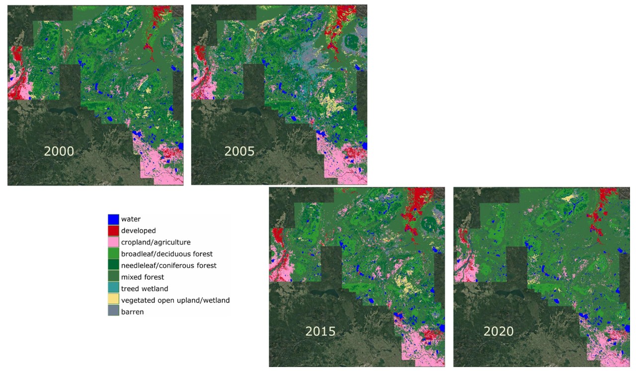
Figure 5: Land use/Land cover maps created by the developed 2010 Random Forest classifier from 2000, 2005, 2015, 2020 at-surface reflectance orthorectified and harmonized Landsat mosaics.

The overall accuracy of the classifier is 96.4 for training and 85.3 for testing sets, while the Cohen’s kappa ranges from 97.7 for training to 82.3 for testing sets, demonstrating the strength of the results derived from the classifier. For the testing set, producer’s accuracies range from 84.8 to 96.9 for six of the classes, but only reach 63.1 for Treed Wetland, 64.3 for Broadleaf Forest and 66.9 for Vegetated Open Upland/Wetland, suggesting that there are limitations in the classifier’s ability to differentiate across classes. User’s accuracies range from 80.0 to 96.1, except for Broadleaf Forest, with 70.2, which indicates that most land cover was correctly classified.

The same 2010 RF classifier was then applied to the 2000, 2005, 2015 and 2020 Landsat images to create the temporal LULC maps for subsequent use in the landscape metrics analyses. They are presented in Figure 5. Accuracy assessment on the classified maps was performed using the same set of 2010 ABMI testing points. Although not ideal, as ABMI discontinued the surveys in 2016 and most of the existing points was surveyed before 2000, this was the only available ground truth dataset.

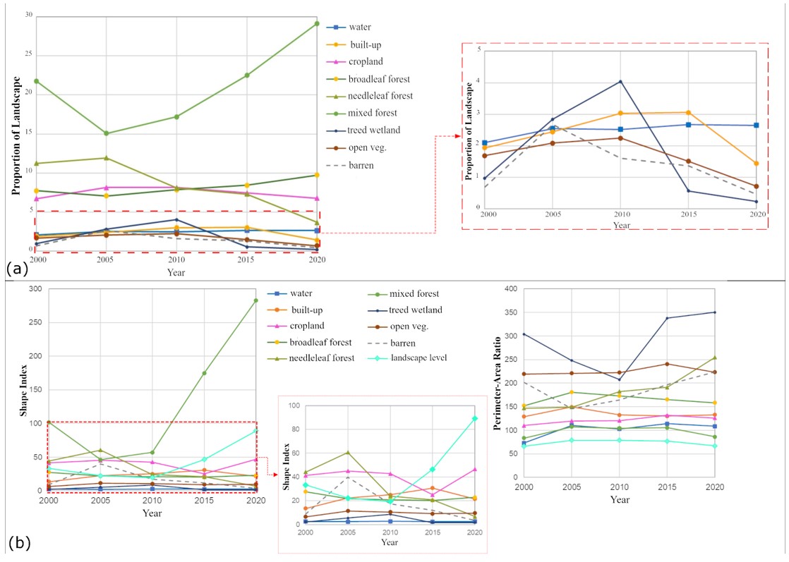
Figure 6: Temporal analysis of the metrics (a) PLAND (proportion of landscape) at the class level and (b) “shape index” and “perimeter-area ratio”, at the class and landscape level

The accuracy assessment was evaluated and is presented in Table 4(b): it shows that the accuracy of the LULC maps is generally consistent over the 2000-2015 period, and declines in 2020, for which ABMI surveys are not available.

5.2 Landscape Metric Selection

Based on correlation analysis and PCA, supported by the literature [8][52] and [53], the three metrics “proportion of landscape” (PLAND), “perimeter-area ratio”, and “shape index” were selected. These metrics (Table 2) were computed for each classified map, and figures were generated for their temporal analysis.

5.3 Temporal Analysis of the Selected Metrics

Figure 6(a) presents the temporal PLAND for each of the nine classes. For the Mixed Forest and Broadleaf Forest classes, the PLAND showed a decrease from 2000 to 2005, followed by an increasing trend from 2005 to 2020. In other words, for the Mixed and Broadleaf Forest classes, the PLAND showed increasing trends of 33% and 36%, respectively, during the study period. The PLAND for the Needleleaf Forest class decreased by 69% from 2005 to 2020 (with an overall decrease of 67% between 2000 and 2020). The Cropland/Agriculture class decreased slightly from 2005 to 2020. The Built-Up class showed an increasing trend of 63% from 2000 to 2010, followed by a 53% decrease from 2015 to 2020. The Treed Wetland, Open Vegetation and Barren classes decreased during the study period.

Figure 6(b) shows the comparison of landscape-level metrics “shape index” and “perimeter-area ratio” (all shown in cyan), with the corresponding class level metrics. Both indices are measures of the complexity of patch geometry, however the shape index is standardized to a basic shape (e.g., ellipse), whereas the perimeter-area index is a simple straightforward measure. At the landscape level, the “shape index” decreased by 41% from 2000 to 2010 and then increased drastically, by 360% from 2010 to 2020. This indicates overall changes in the landscape over the period, which are explained by trends in the class-level metric.

Hence, the decrease in the landscape-level metric was related to the decreased complexity in the geometry of the classes Needleleaf Forest (60% decrease in the class-level metric) and Barren (56% decrease in the class-level metric) from 2005 to 2010. This increase was mainly associated with the increased complexity in the geometry of the class Mixed Forest (390% increase in the class-level metric) from 2010 to 2020. Additionally, the complexity of the geometry of the class Cropland decreased by 54% from 2000 to 2015, followed by an increase of 125% from 2015 to 2020.

At the landscape level, the “perimeter-area ratio” metric barely changed (about 1%) during the study period. However, larger changes were observed at the class level. The metric exhibited the following changes for the pertinent classes: (1) Barren decreased by 28% from 2000 to 2005, then increased by 53% from 2005 to 2020; (2) Needleleaf Forest was practically unchanged between 2000 and 2005, then increased steadily by 73% between 2005 and 2020; (3) Broadleaf Forest increased from 2000 to 2005 and then decrease steadily from 2005 to 2020; and (4) Cropland increased by a modest 14% during the whole study period.

5.4 Temporal Hierarchical Hotspot Analysis

Following the landscape and class level metric results, zonal PLAND were computed on the combined Forest class, i.e., the aggregated Needleleaf, Broadleaf and Mixed classes. Then the hierarchical hotspot analysis was performed on the spectral indices and zonal PLAND ‘Forest’. In this paper, we only present the analyses for NDVI and NDBI. Figure 7 present the HUC10 level polygons that exhibited significant (from 90% confidence) changes within the four 5-year intervals in the OSA for NDVI, NDBI and zonal PLAND ‘Forest’ metric, respectively.

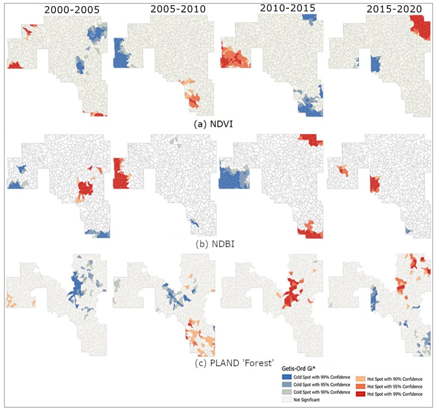
Figure 7: HUC10 level polygons exhibiting positive (in red) and negative (in blue) changes in (a) NDVI (vegetation greenness), (b) NDBI (built-up areas) and, (c) zonal PLAND ‘Forest’ metric over the four 5-year intervals between 2000 and 2020 in the Oil Sands Area

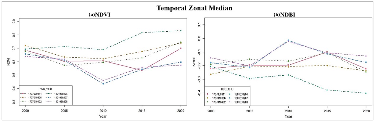
Figure 8: Temporal zonal median graph of NDVI (a) and NDBI (b) for 6 corresponding HUC10 level polygons (whose ID are in legend box) exhibiting significant changes.

Most of the changes occurred in the West, South and North zones of the OSA. The West and South zones correspond to agriculture areas (Figure 4) while the North Zone encompasses urban (Fort McMurray), industry (oil sands) and forest areas (Figure 1). A comparison of Figures 7(a) and 7(b) indicates that the same polygons exhibit opposite changes in NDVI vs. NDBI, suggesting that decreases in vegetation (NDVI) might be associated with increases in NDBI, i.e., built-up or barren land (i.e., bare rock, as opposed to crops or moss, lichen), since these two classes have often similar spectral signatures. The same relationship is suggested by Figure 8, which shows the temporal graphs of the zonal analysis for six HUC10 level polygons that have exhibited changes. This figure also shows that some HUC10 level polygons exhibited very large changes (both positive and negative) while others displayed more subtle changes over time.

Figure 7(c) shows the significant changes affecting zonal PLAND ‘Forest’ at HUC10 level. Interestingly, not all the changes detected by the hierarchical zonal analyses of NDVI and NDBI are visible in zonal PLAND ‘Forest’ and vice versa.

6. Discussion

The OSA is a large and complex area, extending over more than 20 % of the Province of Alberta. To assess environmental change over this extent, we performed a hierarchical zonal analysis, articulated into a double thrust over space and time to identify diverse landscape changes at varying spatial and temporal scales.

The hierarchical time-space zonal analysis may constitute a valuable assessment and management tool, owing to its ability to detect negative changes (i.e., decrease) and positive changes (i.e., increase). Our study shows, for example, localized increases of the vegetation cover that might be associated with reclamation efforts [52]. This study could provide insights into whether changes in boreal forest cover are associated with anthropogenic (industrial activities) or natural (wildfire, insect infestation) environmental stressors. Hence, this study constitutes a starting point to provide information that can support a better understanding not simply of the overall environmental change, but more specifically of the impacts (positive and negative) of industrial activities locally and over time.

The majority of the OSA is covered by boreal forest, with most built-up areas concentrated in the northeast corner of the OSA (Fort McMurray), along the river valley near Peace River, and, to a lesser extent, in the southeast corner (Cold Lake) of the OSA (Figure 1). As well, agricultural land uses are mostly located in the southernmost zone, i.e., the Cold Lake area, and near the Peace River valley. Environmental changes affect these land uses in different ways, hence our class-level analysis identified localized changes in each area. For example, changes to the barren and built-up classes were more significant especially in the Fort McMurray area, whereas changes to the forest class affected the whole OSA, even though changes exhibited opposite signs over time and locally. Landscape metrics and spectral indices were important to evaluate these local and temporal differences (Figures 6, 7, and 8). Landscape metrics provide information on changes not only in landscape composition, i.e., class percentage in each HUC10 level polygon, along with its temporal evolution, but also on its configuration, i.e., on the changes in the fragmentation of the landscape and of individual classes. The metrics selection yielded results consistent with those reported in the literature. Composite measures of “average patch compaction”, “average patch shape”, “perimeter-area” and “large-patch density” were selected [53] while the study of landscape metrics for assessment of land cover change and fragmentation selected five metrics out of nine from their PCA analysis, including “proportion of landscape”, “number of patches”, “largest patch index”, “edge density”, and “landscape shape index” [54].

Spectral indices complemented the landscape metrics analysis. While the metrics focused on the geometric dimension of changes, indices provided substantive information, relating the change to environmental health (e.g., burnt, greenness indices), as well as potentially ascribing them to specific disturbances. Prime examples of a major disturbance are the 2011 Richardson Fire, north of Fort McMurray and the 2016 Fort McMurray wildfire that have significantly altered the landscape [55] and [56]. The decreased reliability of the 2020 LULC classification (Table 4(b)) may be associated with the impact of the 2016 event since the ground truth data for 2020 was not available yet. At the same time, the changes associated with that wildfire are not easily discerned by this analysis, as forested areas were replaced by other type of vegetation, e.g., seedlings, that still appear vegetated in the images. As well, the wildfire occurred near the urban area; hence, some of its effects may be classified simply as urban/barren.

As shown by the hotspot analysis (Figure 7), the main hotspots of change (i.e., contiguous areas characterized by similar changes) occurred in the west zone in the 2000-2005 and 2010-2015 intervals, in the south zone in 2000-2010, and in the north zone (Fort McMurray) in 2015-2020. Interestingly, cold spots (i.e., contiguous areas characterized by negative changes) occurred largely over the same areas as hotspots, but over different time intervals. However, in the central areas of the OSA only cold spots were detected. As shown in Figure 9(c), these synoptic changes appear more sporadic at finer spatial resolution. These results are relative to the initial scale of analysis, as discussed below (paragraph 6.3). For the HUCs that experienced significant changes, a temporal decrease (negative change) in agricultural land use was accompanied by a simultaneous increase (positive change) in built-up or barren areas.

Spatial and temporal extents were dictated by project needs. While the 5-year intervals were determined following the literature discussed in this paper (i.e., [3]-[11]), the HUC level analyses responded to specific project requirements. This said, the presented hierarchical analysis, along with the hotspot analysis, allow transitioning across analytical scales, mindful of the MAUP, and provide a framework for cross-scale analyses applicable to other contexts.

6.1 Limitations and Uncertainties

Our study is necessarily limited by many factors. At the fundamental level, analysis and communication of environmental changes should encompass narratives, images, graphs, statistical and quantitative methods, along with traditional environmental knowledge and other Indigenous ways of knowing [57]. The scope of our project limited our work to the analysis discussed here. Further limitations of this study stem from the sheer size of the study area, and the reliance on data products, derived from remotely sensed images, with their inherent limitations in representing the area under scrutiny. The analysis presented in this paper provided some strategies to mitigate some of these limitations, by (1) using a hierarchical approach that investigates only areas subject to change and (2) providing some analytical redundancy (double thrust) to compensate for data and classification limitations. However, we recognize that our approach suffers from the inherent limitations of scales, computational power, and assumptions.

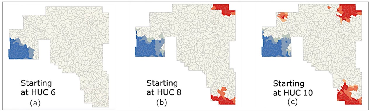
Figure 9: Hierarchical zonal analysis of NDBI between 2010 and 2015 at the finest (HUC10) level, exhibiting positive (red) and negative (blue) changes
(a) HUC6 level (b) HUC8 level (c) HUC10 level.

6.2 Landsat Mosaic and LULC Classification

To create the Landsat images for the period of the study, the median of the orthorectified and at-surface reflectance Landsat collections (Collection 1) over the growing season was selected: this portion of the year was chosen because it is generally the time when the OSA is as cloudless as possible. To obtain cloudless and gapless imagery, multi-date scenes from a range of months were mosaicked together, although vegetation phenology (levels) may vary through those months. However, there is no evidence that this limitation impacts the hierarchical zonal analysis due to the analysis scale (i.e., HUC10 polygons) nor the comparison of the temporal images.

Validation of the LULC classification was limited by data availability. ABMI reference data are available from discontinuous surveys and varying points. Despite the temporal mismatch, the 2010 dataset performed better than any other set, as it contained the largest sample. As an alternative to ABMI, the Land Cover of Canada for the pertinent years was considered; however, the accuracy and sample size are reported for the entire Canada, with no indication of the sample size and properties for the OSA and 2020 classification map did not exist.

6.3 Modifiable Areal Unit Problem

The modifiable areal unit problem (MAUP), well known in the spatial analytical literature [17], can be summarized in the change in analytical results deriving from changes in the spatial units used in the analysis. This study was conducted at nested scales, and we are mindful that results obtained at each scale cannot be directly inferred to other scales, as exemplified by Figure 9. Likewise, results obtained for HUC polygons cannot be inferred to other spatial units. Further, some analytical routines may be impacted by edge effects, as shown in Figure 10, which tend to occur when unusually high or low values occur near the edges of the study area, impacting local analytical results in that area [58].

Moreover, our study gave evidence of a difference in results associated with analyses conducted on a single merged region (Figure 10(b)) as opposed to its constituent portions (Figure 10(a)). We can speculate that this was the result of the combined edge effects and MAUP problems. While there exist corrections for edge effects, it is known that the MAUP has no solution. Therefore, we can only point out to this finding and caution about this occurrence in studies similar to this one.

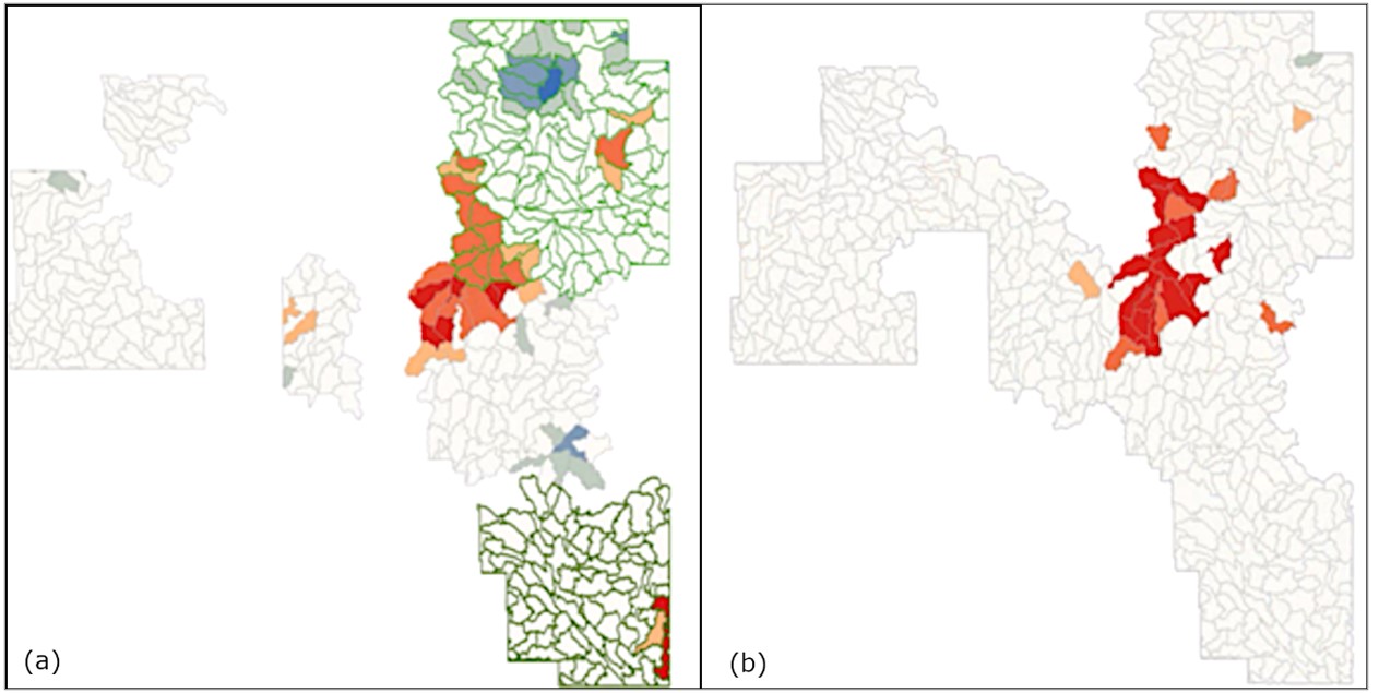
Figure 10: Hierarchical zonal analysis of zonal PLAND ‘Forest’ between 2010 and 2015 where the zonal analysis has been done on each zone of interest (6 zones) separately (a) or on the merged zones (1 zone) covering the OSA (b) where HUC10 level polygons are exhibiting positive (red) and negative (blue) changes. On (a), the north and south zones of interest have been highlighted in light and dark green respectively to show that they were analysed separately.